Distribution Federate Implementation

Distribution Federate Implementation#

This file is the distribution simulation federate file. It controls the simulation of the distribution system. The code includes the distribution network power flow simulation and the interface of data exchange with other simulators such as the transmission simulator.

Steps to configure a Distribution Federate

Broker already initialized in Transmission federate, so it is not needed.
Creating a federate with information.
Enlist publication and subscription items
Load system data (DSS file) for distribution system simulation
Fix simulation step and time for co-simulaiton
Run co-simulation

Simulator OpenDSS has been used as a simulator for distribution systems through the Python wrapper OpenDSSDirect.py, which enables direct interaction with the OpenDSS engine without requiring the COM interface. This makes it faster and more compatible across different platforms [1]. It provides a functional API for executing OpenDSS commands and retrieving data, making it well-suited for integration with data science tools like Pandas and NumPy.
Methodology The total load of the IEEE 34-bus distribution system varies with a standard deviation of 2.5%. The varied load is published so that it gets reflected in the transmission system. When the transmission federate runs the simulation, it will use the updated load from the distribution system. Since the total load of the 34-bus distribution system does not match the load at Bus 4 of the IEEE-14 transmission system, it must be scaled.

Running Transmission_Federat and Distribution_Federate simultaneously

To run the co-simulation, we must run Transmission_Federate.ipynb & Distrubtion_Federate.ipynb together (run all cells at once).

Import helics and openDSSDirect.

If helics has not been installed, run !pip install helics inside a cell.
If OpenDSSDirect.py has not been installed, run !pip OpenDSSDirect.py inside a cell.

import os
import sys
import numpy as np
import helics as h
import opendssdirect as dss
from opendssdirect.utils import run_command
import csv
import pandas as pd
import matplotlib.pyplot as plt

Here, we directly create a distribution federate, as the broker has already been created in the transmission federate.

Create a Distribution Federate info object#

federate_name=’34Bus’ fedinfo = h.helicsCreateFederateInfo() h.helicsFederateInfoSetCoreName(fedinfo, f”{federate_name}”) h.helicsFederateInfoSetCoreTypeFromString(fedinfo, “zmq”) h.helicsFederateInfoSetCoreInitString(fedinfo, “–federates=1”) h.helicsFederateInfoSetTimeProperty(fedinfo, h.helics_property_time_delta, 0.01)

Create Value Federate#

fed = h.helicsCreateValueFederate(f”{federate_name}”, fedinfo) print(f”{federate_name}: Value federate created”, flush=True)

PUBLICATIONS = {}
SUBSCRIPTIONS = {}
publications= {
      "sourcebus/TotalPower": {
      "element_name": "sourcebus",
      "element_type": "Bus",
      "topic": "Totalpower",
      "type": "complex",
      "value": "Power",
      "unit": "kva",
      "fold": "sum"
    }
  }
subscriptions= {
    "sourcebus/pu": {
      "element_name": "sourcebus",
      "element_type": "Bus",
      "topic": "TransmissionSim/Voltage_4",
      "required": True,
      "key": "TransmissionSim/transmission_voltage",
      "type": "complex",
      "unit": "pu",
      "value": "Voltage"
    }
  }

for k, v in publications.items():
    pub = h.helicsFederateRegisterTypePublication(fed, v["topic"], "complex", "")
    PUBLICATIONS[k] = pub
for k, v in subscriptions.items():
    sub = h.helicsFederateRegisterSubscription(fed, v["topic"], "")
    SUBSCRIPTIONS[k] = sub

Entering execution#

h.helicsFederateEnterExecutingMode(fed) print(f”{federate_name}: Entering execution mode”, flush=True)

Load the IEEE 34-bus distribution system files for simulation. OpenDSS is used for the distribution system simulation. A 2.5% standard deviation in load variation has been introduced for the simulation period, which will be reflected on the transmission side. Scaling is applied to adjust the total load of the 34-bus system to make it equivalent to the load at the bus in the transmission system.

## Load DSS file and initial simulation

feeder_name = '34Bus'
path34 = os.getcwd()
consistent_random_object = np.random.RandomState(981)
load_profile_random = consistent_random_object.normal(1,0.025, 15) #0.02
print('------ Running the {} feeder in opendss'.format(feeder_name))

print(path34)
run_command(f'compile "{os.path.join(path34, "DSSfiles", "Master.dss")}"')

if dss.Text.Result() == '':
    print('------ Success for the test run -----')
else:
    print('------ Opendss failed ----')
    print(f'Error is "{dss.Text.Result()}"!')
run_command("BatchEdit Load..* Vminpu=0.9")
run_command("New Loadshape.dummy npts=60 sinterval=1 Pmult=[file=dummy_profile.txt]")
run_command("BatchEdit Load..* Yearly=dummy")
run_command("set mode=yearly number=60 stepsize=1s")
dss.Solution.ControlMode(2)
print(f"dss.Solution.Mode()={dss.Solution.Mode()}")
print(f"dss.Solution.ControlMode()={dss.Solution.ControlMode()}")

BASEKV = dss.Vsources.BasekV()
loadname_all=[]
loadkw_all=[]
loadkvar_all=[]
num_loads = dss.Loads.Count()
dss.Loads.First()
for i in range(num_loads):
    loadname = dss.Loads.Name()
    loadkw = dss.Loads.kW()
    loadkvar = dss.Loads.kvar()
    loadname_all.append(loadname)
    loadkw_all.append(loadkw)
    loadkvar_all.append(loadkvar)
    dss.Loads.Next()
print(f"Total power base line is {dss.Circuit.TotalPower()}")
base_load = abs(dss.Circuit.TotalPower()[0])
loadkw_dict = dict(zip(loadname_all, loadkw_all))
loadkvar_dict = dict(zip(loadname_all, loadkvar_all))
allnodenames = dss.Circuit.AllNodeNames()
num_nodes = len(allnodenames)
os.chdir(path34)

------ Running the 34Bus feeder in opendss
/home/hcui9/repos/powercybertraining.github.io/pct/modules/06
------ Success for the test run -----
dss.Solution.Mode()=2
dss.Solution.ControlMode()=2
Total power base line is [-970.6704185860139, -150.43653562121725]

/tmp/ipykernel_53976/3687056038.py:8: DeprecationWarning: run_command is deprecated (use Command, Commands or the callable shortcut), see https://github.com/dss-extensions/OpenDSSDirect.py/issues/70
  run_command(f'compile "{os.path.join(path34, "DSSfiles", "Master.dss")}"')
/tmp/ipykernel_53976/3687056038.py:15: DeprecationWarning: run_command is deprecated (use Command, Commands or the callable shortcut), see https://github.com/dss-extensions/OpenDSSDirect.py/issues/70
  run_command("BatchEdit Load..* Vminpu=0.9")
/tmp/ipykernel_53976/3687056038.py:16: DeprecationWarning: run_command is deprecated (use Command, Commands or the callable shortcut), see https://github.com/dss-extensions/OpenDSSDirect.py/issues/70
  run_command("New Loadshape.dummy npts=60 sinterval=1 Pmult=[file=dummy_profile.txt]")
/tmp/ipykernel_53976/3687056038.py:17: DeprecationWarning: run_command is deprecated (use Command, Commands or the callable shortcut), see https://github.com/dss-extensions/OpenDSSDirect.py/issues/70
  run_command("BatchEdit Load..* Yearly=dummy")
/tmp/ipykernel_53976/3687056038.py:18: DeprecationWarning: run_command is deprecated (use Command, Commands or the callable shortcut), see https://github.com/dss-extensions/OpenDSSDirect.py/issues/70
  run_command("set mode=yearly number=60 stepsize=1s")

Main Loop for Co-simulation#

This is the main loop for co-simulation. It runs the distribution system simulation at each given time step. The publication of active and reactive power and the subscription to voltage magnitude and angle occur simultaneously until the loop terminates.

dss.Vsources.PU(1.01)
scale = 0.478*100/0.970657
total_time=15
simulation_step_time=1
current_time=0
V_mag=[]
V_ang=[]
load_var=[]
time_list=[]
for request_time in np.arange(0, total_time, simulation_step_time):
    while current_time < request_time:
        current_time = h.helicsFederateRequestTime(fed, request_time)
    print(f"current_time={current_time}")
    dss.run_command("Solve number=1 stepsize=1s")
    allbusmagpu = dss.Circuit.AllBusMagPu()
    S = dss.Circuit.TotalPower() 
    print(f"Total power={dss.Circuit.TotalPower()}")
    print(f"Overall after adjustment S={S}")
    P = -S[0]
    Q = -S[1]

    P = P*scale
    Q = Q*scale
    h.helicsPublicationPublishComplex(pub, P, Q)
    print("Sent Active power at time {}: {} kw".format(current_time, P))
    print("Sent Reactive power at time {}: {} kvar".format(current_time, Q))
    print("=============================")
    for key, sub in SUBSCRIPTIONS.items():
        val = h.helicsInputGetComplex(sub)
        if subscriptions[key]['value'] == 'Voltage':

            print("Received voltage mag at time {}: {} pu".format(current_time, val.real))
            print("Received voltage ang at time {}: {} rad".format(current_time, val.imag))

            voltage, angle_rad = val.real,val.imag
            angle_deg = np.degrees(angle_rad)
            if current_time == 0:
                print('manually set up first step voltage')
                angle_deg = 0
                voltage = 1
            dss.Vsources.AngleDeg(angle_deg)
            dss.Vsources.PU(voltage)
    V_mag.append(voltage)
    V_ang.append(angle_rad)
    time_list.append(current_time)
    load_var.append(dss.Circuit.TotalPower())
    dss.Loads.First()
    for j in range(num_loads):
        loadname = dss.Loads.Name()
        load_mult = load_profile_random[int(current_time)]
        loadkw_new = load_mult * loadkw_dict[loadname]
        loadkvar_new = load_mult * loadkvar_dict[loadname]
        run_command('edit load.{ln} kw={kw}'.format(ln=loadname, kw=loadkw_new))
        run_command('edit load.{ln} kvar={kw}'.format(ln=loadname, kw=loadkvar_new))
        dss.Loads.Next()

h.helicsFederateDestroy(fed)
print('Federate finalized')

current_time=0
Total power=[-970.6902667097943, -150.45499436296086]
Overall after adjustment S=[-970.6902667097943, -150.45499436296086]
Sent Active power at time 0: 47801.63821898793 kw
Sent Reactive power at time 0: 7409.155582816102 kvar
=============================
Received voltage mag at time 0: -1e+49 pu
Received voltage ang at time 0: 0.0 rad
manually set up first step voltage
current_time=1.0
Total power=[-904.7684976790478, -83.902540987507]
Overall after adjustment S=[-904.7684976790478, -83.902540987507]
Sent Active power at time 1.0: 44555.32097235016 kw
Sent Reactive power at time 1.0: 4131.780288199471 kvar
=============================
Received voltage mag at time 1.0: 1.0114034500520985 pu
Received voltage ang at time 1.0: -0.07696511657375282 rad
current_time=2.0
Total power=[-993.7380620108355, -178.12353883450336]
Overall after adjustment S=[-993.7380620108355, -178.12353883450336]
Sent Active power at time 2.0: 48936.62680444064 kw
Sent Reactive power at time 2.0: 8771.692942295023 kvar
=============================
Received voltage mag at time 2.0: 1.011401794902155 pu
Received voltage ang at time 2.0: -0.0770189711690463 rad
current_time=3.0
Total power=[-988.2223283692978, -170.78225516654936]
Overall after adjustment S=[-988.2223283692978, -170.78225516654936]
Sent Active power at time 3.0: 48665.00452379412 kw
Sent Reactive power at time 3.0: 8410.171458054761 kvar
=============================
Received voltage mag at time 3.0: 1.0150319198052244 pu
Received voltage ang at time 3.0: 0.0354939385936789 rad
current_time=4.0
Total power=[-967.1785366246238, -134.7297139850706]
Overall after adjustment S=[-967.1785366246238, -134.7297139850706]
Sent Active power at time 4.0: 47628.703085288646 kw
Sent Reactive power at time 4.0: 6634.7642148424975 kvar
=============================
Received voltage mag at time 4.0: 1.0102754291179836 pu
Received voltage ang at time 4.0: 0.11940578933267289 rad

/tmp/ipykernel_53976/2529339107.py:14: DeprecationWarning: run_command is deprecated (use Command, Commands or the callable shortcut), see https://github.com/dss-extensions/OpenDSSDirect.py/issues/70
  dss.run_command("Solve number=1 stepsize=1s")
/tmp/ipykernel_53976/2529339107.py:53: DeprecationWarning: run_command is deprecated (use Command, Commands or the callable shortcut), see https://github.com/dss-extensions/OpenDSSDirect.py/issues/70
  run_command('edit load.{ln} kw={kw}'.format(ln=loadname, kw=loadkw_new))
/tmp/ipykernel_53976/2529339107.py:54: DeprecationWarning: run_command is deprecated (use Command, Commands or the callable shortcut), see https://github.com/dss-extensions/OpenDSSDirect.py/issues/70
  run_command('edit load.{ln} kvar={kw}'.format(ln=loadname, kw=loadkvar_new))

current_time=5.0
Total power=[-980.706719023312, -163.2222531807627]
Overall after adjustment S=[-980.706719023312, -163.2222531807627]
Sent Active power at time 5.0: 48294.89837225128 kw
Sent Reactive power at time 5.0: 8037.879191146261 kvar
=============================
Received voltage mag at time 5.0: 1.009309107624471 pu
Received voltage ang at time 5.0: 0.08214034804250755 rad
current_time=6.0
Total power=[-945.5609523511259, -118.32983772134871]
Overall after adjustment S=[-945.5609523511259, -118.32983772134871]
Sent Active power at time 6.0: 46564.14523604509 kw
Sent Reactive power at time 6.0: 5827.152375226747 kvar
=============================
Received voltage mag at time 6.0: 1.010959796425234 pu
Received voltage ang at time 6.0: 0.040318443544884376 rad
current_time=7.0
Total power=[-989.9663227952136, -174.06903097687848]
Overall after adjustment S=[-989.9663227952136, -174.06903097687848]
Sent Active power at time 7.0: 48750.88752217437 kw
Sent Reactive power at time 7.0: 8572.028719408392 kvar
=============================
Received voltage mag at time 7.0: 1.010978721780115 pu
Received voltage ang at time 7.0: 0.010421818404916218 rad
current_time=8.0
Total power=[-948.3151480537706, -118.36095074703863]
Overall after adjustment S=[-948.3151480537706, -118.36095074703863]
Sent Active power at time 8.0: 46699.77559217132 kw
Sent Reactive power at time 8.0: 5828.684536049755 kvar
=============================
Received voltage mag at time 8.0: 1.01296187898716 pu
Received voltage ang at time 8.0: 0.035006979449757565 rad
current_time=9.0
Total power=[-1012.2917825599592, -199.39412347995815]
Overall after adjustment S=[-1012.2917825599592, -199.39412347995815]
Sent Active power at time 9.0: 49850.30469709285 kw
Sent Reactive power at time 9.0: 9819.16279627304 kvar
=============================
Received voltage mag at time 9.0: 1.0107093324628642 pu
Received voltage ang at time 9.0: 0.04652199139537953 rad
current_time=10.0
Total power=[-970.4838082702672, -148.62588442768757]
Overall after adjustment S=[-970.4838082702672, -148.62588442768757]
Sent Active power at time 10.0: 47791.47117397677 kw
Sent Reactive power at time 10.0: 7319.081071525231 kvar
=============================
Received voltage mag at time 10.0: 1.012374039405704 pu
Received voltage ang at time 10.0: 0.06667494695734988 rad
current_time=11.0
Total power=[-988.6776777663633, -169.2703405598685]
Overall after adjustment S=[-988.6776777663633, -169.2703405598685]
Sent Active power at time 11.0: 48687.42820299258 kw
Sent Reactive power at time 11.0: 8335.717229424723 kvar
=============================
Received voltage mag at time 11.0: 1.009302622310051 pu
Received voltage ang at time 11.0: 0.029027350996189562 rad
current_time=12.0
Total power=[-965.8915994849767, -145.57301106470365]
Overall after adjustment S=[-965.8915994849767, -145.57301106470365]
Sent Active power at time 12.0: 47565.327871103684 kw
Sent Reactive power at time 12.0: 7168.7423352356545 kvar
=============================
Received voltage mag at time 12.0: 1.0112396674958422 pu
Received voltage ang at time 12.0: -0.02721157995253078 rad
current_time=13.0
Total power=[-942.3427567841911, -109.76918889728627]
Overall after adjustment S=[-942.3427567841911, -109.76918889728627]
Sent Active power at time 13.0: 46405.665208497274 kw
Sent Reactive power at time 13.0: 5405.583258854862 kvar
=============================
Received voltage mag at time 13.0: 1.011012686834132 pu
Received voltage ang at time 13.0: -0.06752358126897155 rad
current_time=14.0
Total power=[-986.6654366250386, -169.5576545157085]
Overall after adjustment S=[-986.6654366250386, -169.5576545157085]
Sent Active power at time 14.0: 48588.335396207774 kw
Sent Reactive power at time 14.0: 8349.866004006426 kvar
=============================
Received voltage mag at time 14.0: 1.012172383185296 pu
Received voltage ang at time 14.0: -0.07816487781033815 rad
Federate finalized

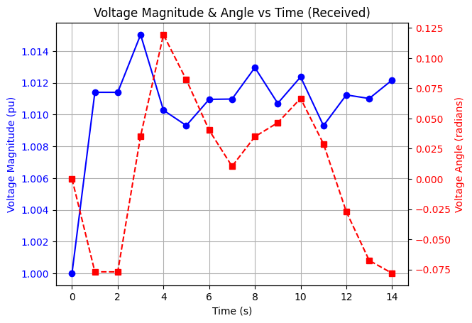
Here we plot the voltage magnitude and angle received from Transmission Federate.

import matplotlib.pyplot as plt
import matplotlib
%matplotlib inline
fig, ax1 = plt.subplots(figsize=(6.4, 4.8))
ax1.plot(time_list, V_mag, label="Voltage Magnitude (pu)", marker='o', linestyle='-', color='b')
ax1.set_xlabel("Time (s)")
ax1.set_ylabel("Voltage Magnitude (pu)", color='b')
ax1.tick_params(axis='y', labelcolor='b')
ax2 = ax1.twinx()
ax2.plot(time_list, V_ang, label="Voltage Angle (radians)", marker='s', linestyle='--', color='r')
ax2.set_ylabel("Voltage Angle (radians)", color='r')
ax2.tick_params(axis='y', labelcolor='r')
plt.title("Voltage Magnitude & Angle vs Time (Received)")
ax1.grid(True)
plt.show()

../../_images/253d523a0c2e17388b52585c6014fd7afccf2cb044b2b16c1479f2f503724d2f.png

Result Analysis#

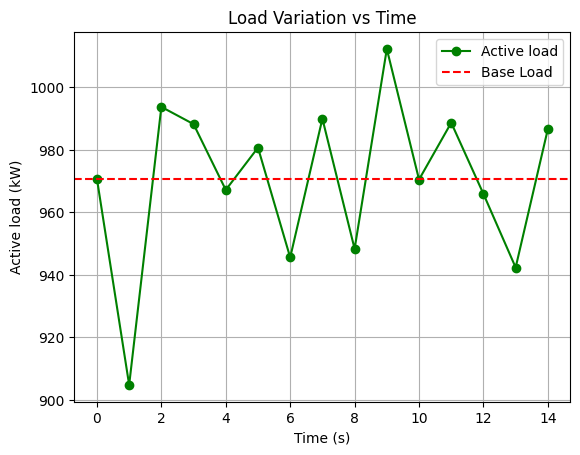
The distribution federate starts to receive the voltage angle and magnitude at 1 second. After sending the varying P & Q signals to the transmission federate, it receives the updated voltage value from the transmission federate based on the simulation results. The load variation on the distribution side is reflected on the transmission side, which causes a change in the voltage at bus 4 of the transmission system, to which the distribution feeder is connected.

Here, we plot the total active load variation of the IEEE-34 bus distribution system over the simulation period.

import matplotlib.pyplot as plt
%matplotlib inline
P_var = [abs(sublist[0]) for sublist in load_var]
plt.figure(figsize=(6.4, 4.8))
plt.plot(time_list, P_var, label="Active load", marker='o', linestyle='-', color='g')
plt.axhline(base_load, color='r', linestyle='--', label=f"Base Load")  # Horizontal line for base load

plt.xlabel("Time (s)")
plt.ylabel("Active load (kW)")
plt.title("Load Variation vs Time")
plt.legend()
plt.grid(True)
plt.show()

../../_images/bf3c4809a53ae2da68cc599e9b2b100cbf56e811e93243c20c8523b3ae270031.png

References#

“OpenDSSDirect.py — OpenDSSDirect.py 0.9.1 documentation,” Dss-extensions.org, 2017. https://dss-extensions.org/OpenDSSDirect.py/ (accessed Feb. 16, 2025).
OpenDSS Documentation: https://www.epri.com/pages/sa/opendss
Montenegro, D., and Dugan, R. “OpenDSS and OpenDSS-PM open source libraries for NI LabVIEW.” 2017 IEEE Workshop on Power Electronics and Power Quality Applications (PEPQA), 2017.